

Local Search Algorithms in Artificial Intelligence are optimization techniques that improve a solution by repeatedly moving to a better neighbouring state. Instead of exploring every possible path, they focus on finding efficient and practical solutions for complex problems.
- Improve solutions through neighbouring states
- Useful for optimization and decision-making problems
- Commonly used in scheduling, routing and machine learning tasks
Basic Terminologies
- State: A possible solution to the problem
- Current State: The solution currently being evaluated
- Neighbour State: A solution formed by making small changes to the current state
- Objective Function: A function used to measure the quality of a solution
- Local Optimum: The best solution among nearby states
- Global Optimum: The best possible solution in the entire search space
Working
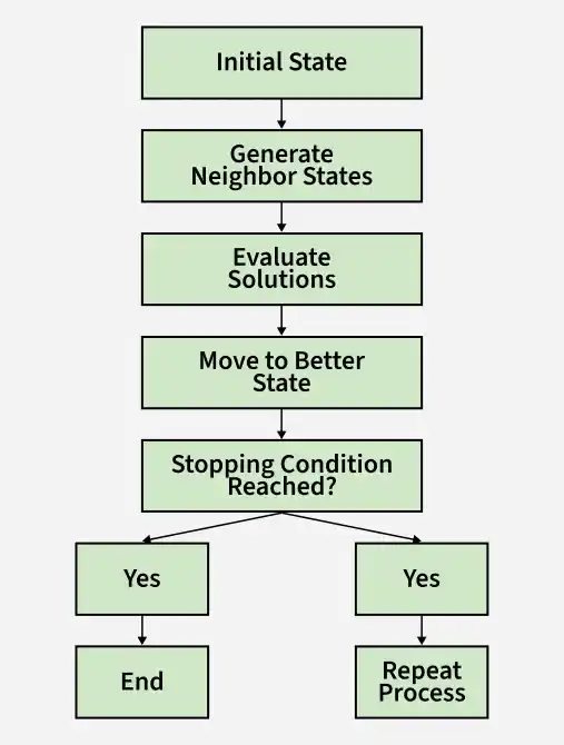
1. Pick a starting point: Start with a possible solution which is often random but sometimes based on rule.
2. Find the Neighbours:
- Neighbours are similar solutions we can get by making small, simple changes to the current one.
- For example, in a puzzle, swapping two pieces creates a neighbour.
3. Compare: Look around at all neighbors to see if any are better.
4. Move: If a better neighbor exists, move to it, making it our new “current” solution.
5. Repeat: Keep searching from the new point, following the same steps.
6. Stop: When none of the neighbors are better or after enough tries.
Types of Local Search Algorithms
1. Hill-Climbing Search Algorithm
Hill-Climbing search algorithm is a simple local search algorithm that continuously moves toward a better neighboring solution until no improvement is possible.
Process:
- Start: Begin with an initial solution.
- Evaluate: Assess the neighboring solutions.
- Move: Transition to the neighbor with the highest objective function value if it improves the current solution.
- Repeat: Continue this process until no better neighboring solution exists.
Pros:
- Easy to implement.
- Works well in small or smooth search spaces.
Cons:
- May get stuck in local optima.
- Limited exploration of the search space.
import random

def f(x):
    return - (x - 3)**2 + 5

def hill_climb():
    current_x = random.uniform(0, 6)
    step_size = 0.1
    max_iterations = 100
    for i in range(max_iterations):
        neighbors = [current_x + step_size, current_x - step_size]
        neighbors = [x for x in neighbors if 0 <= x <= 6]
        neighbor_scores = [f(x) for x in neighbors]
        best_neighbor_idx = neighbor_scores.index(max(neighbor_scores))
        best_neighbor = neighbors[best_neighbor_idx]
        if f(best_neighbor) > f(current_x):
            current_x = best_neighbor
        else:
            break
    return current_x, f(current_x)

result_x, result_value = hill_climb()
print(f"Found maximum at x = {result_x:.2f}, value = {result_value:.2f}")
Output:
Found maximum at x = 3.02, value = 5.00
2. Simulated Annealing
Simulated Annealing is a local search algorithm inspired by the heating and cooling process in metallurgy. It occasionally accepts worse solutions to escape local optima, with the acceptance probability decreasing over time.
Process:
- Start: Begin with an initial solution and an initial temperature.
- Move: Transition to a neighboring solution with a certain probability.
- Cooling Schedule: Gradually reduce the temperature over time.
- Probability Function: Accept worse solutions with decreasing probability as temperature lowers.
Pros:
- Helps escape local optima due to probabilistic acceptance of worse solutions.
- Explores the search space more effectively.
Cons:
- Requires careful parameter tuning.
- Computationally expensive due to repeated evaluations.
import math
import random

def f(x):
    return - (x - 3)**2 + 5

def get_neighbor(x, step_size=0.1):